Abstract
PDE-constrained optimization problems arise in a wide range of scientific and engineering applications, including aerodynamic design, heat transfer, and inverse problems. The dominant computational cost in these problems stems from repeatedly solving large linear systems associated with discretized state and adjoint equations. Quantum linear system algorithms (QLSAs) offer exponential speedups with respect to the dimension of such systems under suitable assumptions, but their applicability to classical scientific computing is limited by the need to extract full classical solutions. In this work, we present a hybrid quantum--classical optimization framework that integrates the classical adjoint method with QLSA-based adjoint solves and swap-test-based inner product estimation. By computing reduced gradients without reconstructing the full adjoint vector, the proposed approach avoids quantum tomography and preserves the theoretical quantum advantage. By replacing the classical adjoint linear solve with a quantum solver, the complexity of our approach exhibits exponential speed-up with respect to number of state variables. Our algorithm is tested numerically using Qiskit.
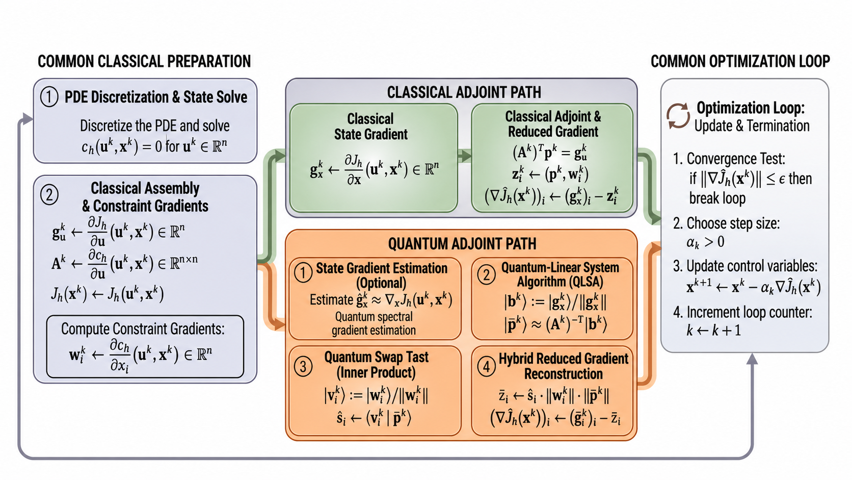
The central idea of this work is to accelerate gradient evaluation in PDE-constrained optimization by replacing the classical adjoint linear solve with a quantum linear system algorithm (QLSA).
Throughout, u denotes the PDE state variable and x denotes the control variable. In classical adjoint-based optimization, the adjoint variable p is obtained by solving the linear system
$$ A^T p = \frac{\partial J}{\partial u}(u,x) $$where \(A = \partial c/\partial u\) is the Jacobian of the discretized PDE constraint with respect to the state, and \(J(u,x)\) is the objective functional.
Once the adjoint vector is computed, the reduced gradient of the objective with respect to the control variables is given by
$$ (\nabla \hat{J}(x))_i = \frac{\partial J}{\partial x_i} - \left\langle p,\frac{\partial c}{\partial x_i} \right\rangle . $$The proposed hybrid quantum–classical method prepares the adjoint state using a quantum linear system algorithm
$$ |p\rangle \propto A^{-T} g_u , $$where \(g_u = \partial J / \partial u\). Instead of reconstructing the full adjoint vector, the algorithm computes the required inner products directly using quantum swap-test measurements. This avoids quantum state tomography and allows the reduced gradient to be estimated while preserving the potential quantum speedup of the linear-system solve.
Method Overview
- Initialize: choose an initial control \(x^0\).
- State solve (classical): solve the discretized PDE \[ c(u^k,x^k)=0 \] to obtain the state \(u^k\).
- Objective evaluation: compute the reduced objective \[ \hat J(x^k)=J(u^k,x^k). \]
- Derivative assembly: form the Jacobian \[ A^k=\frac{\partial c}{\partial u}(u^k,x^k) \] and the state gradient \[ g_u^k=\frac{\partial J}{\partial u}(u^k,x^k). \]
- Quantum adjoint solve: prepare the adjoint state \[ |p^k\rangle \propto (A^k)^{-T} g_u^k \] using a quantum linear system algorithm.
- Gradient estimation: estimate \[ \left\langle p^k,\frac{\partial c}{\partial x_i}\right\rangle \] for each control variable using swap-test measurements.
- Control update: update the control \[ x^{k+1}=x^k-\alpha_k\nabla\hat J(x^k). \]
- Repeat until convergence.
Ignoring lower-order terms, the per-iteration runtime is dominated by:
\[ T_{\text{iter}} = O\!\left( (m+1)\, s\, n_u\, \kappa \log\!\frac{1}{\varepsilon_s} \;+\; n_x n_u \;+\; \varepsilon_{\text{spectral}}^{-1} \;+\; n_x\,\log(n_u)\, s^2 \kappa^2\, \varepsilon_{\text{swap}}^{-2}\varepsilon_{\text{adjoint}}^{-1} \right). \](First term: classical state solves + line search. Middle terms: classical derivative assembly and the optional quantum spectral gradient estimate. Last term: quantum adjoint preparation and swap-test gradient estimation, repeated for each of the \(n_x\) control variables.)
Notation.
- nu – number of state variables (grid unknowns in the PDE discretization)
- nx – number of control variables in the optimization problem
- s – sparsity of the Jacobian matrix (maximum number of nonzero entries per row)
- κ – denotes an upper bound on the condition number of the state Jacobian
- εs – tolerance used for the classical Krylov solver in the state equation
- εspectral – accuracy of the (optional) quantum spectral control-gradient estimate
- εadjoint – accuracy to which the QLSA prepares the adjoint state
- εswap – additive error of the swap-test inner-product estimate
- m – maximum number of additional state solves performed during the line search
A1. The reduced objective \( \hat{J}_h : \mathbb{R}^{n_x} \to \mathbb{R} \) is continuously differentiable and bounded below.
A2. The gradient \( \nabla \hat{J}_h \) is Lipschitz continuous.
A3. The inexact reduced gradient satisfies
\[ \|e^k\|_2 \le \rho \, \|\nabla \hat{J}_h(x^k)\|_2 . \]A4. The step sizes \( \alpha_k \) satisfy the bounded step-size conditions of Lemma 5.3.
Result. Under these assumptions
\[ \lim_{k\to\infty}\|\nabla \hat{J}_h(x^k)\|_2 = 0 , \]and every accumulation point of \(x^k\) is a critical point of \( \hat{J}_h \).
Experiments and Results
We consider two PDE-constrained optimization experiments. The first is a heat equation ,
\[ -\kappa\,u''(y) + \epsilon(u)\bigl(u^4-T_\infty^4\bigr) + h\bigl(u-T_\infty\bigr) = Bx, \qquad u(0)=u(1)=0, \]with objective
\[ J(u,x)=\frac12\|u-u_d\|^2+\frac{\beta}{2}\|x\|^2. \]The second is an elliptic equation
\[ -\bigl(\kappa(x)u'(x)\bigr)' + c(x)u(x) = Bx+f(x), \qquad u(0)=u(1)=0, \]with objective
\[ J(u,x)=\frac12\|u-u_d\|^2+\frac{\alpha}{2}\|x\|^2. \]Both experiments are discretized by finite differences and used to compare classical and hybrid methods.
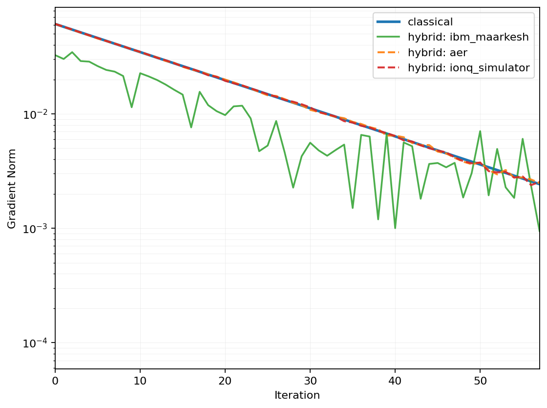
Gradient-norm convergence on the heat-equation problem (nu=4 state variables,
nx=2 control variables), comparing the fully classical adjoint solve
against the hybrid solver run on the Aer simulator, the IonQ simulator, and real IBM Quantum hardware
(ibm_marrakesh). The Aer and IonQ simulator runs track the classical curve almost exactly;
the real-hardware run follows the same overall descent despite the added shot noise of present-day
quantum hardware.
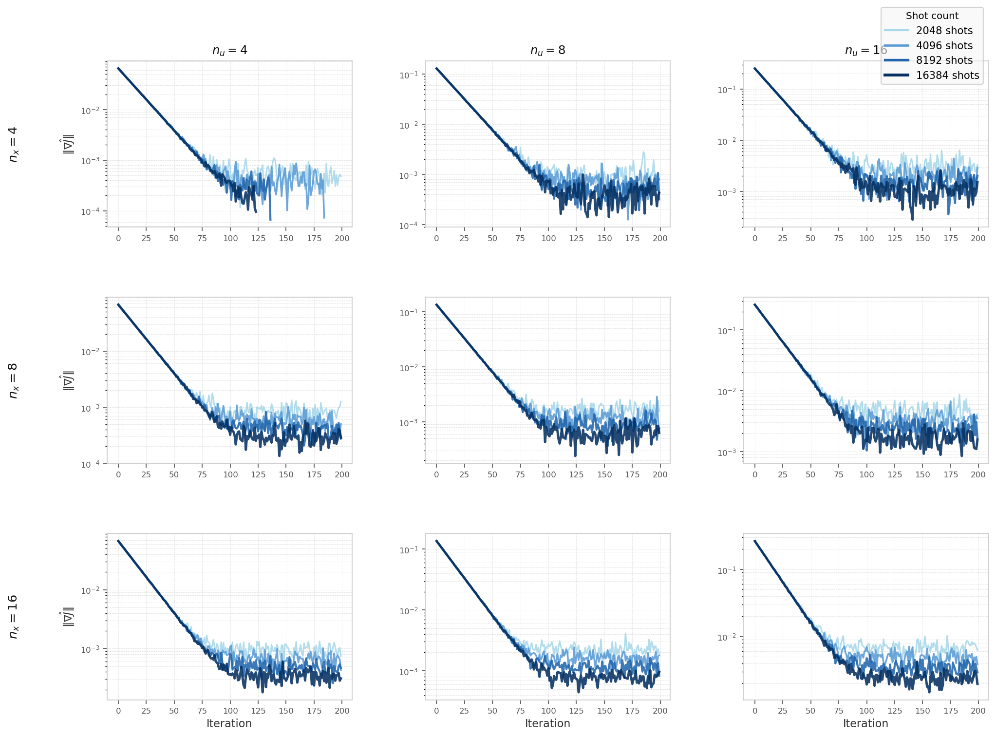
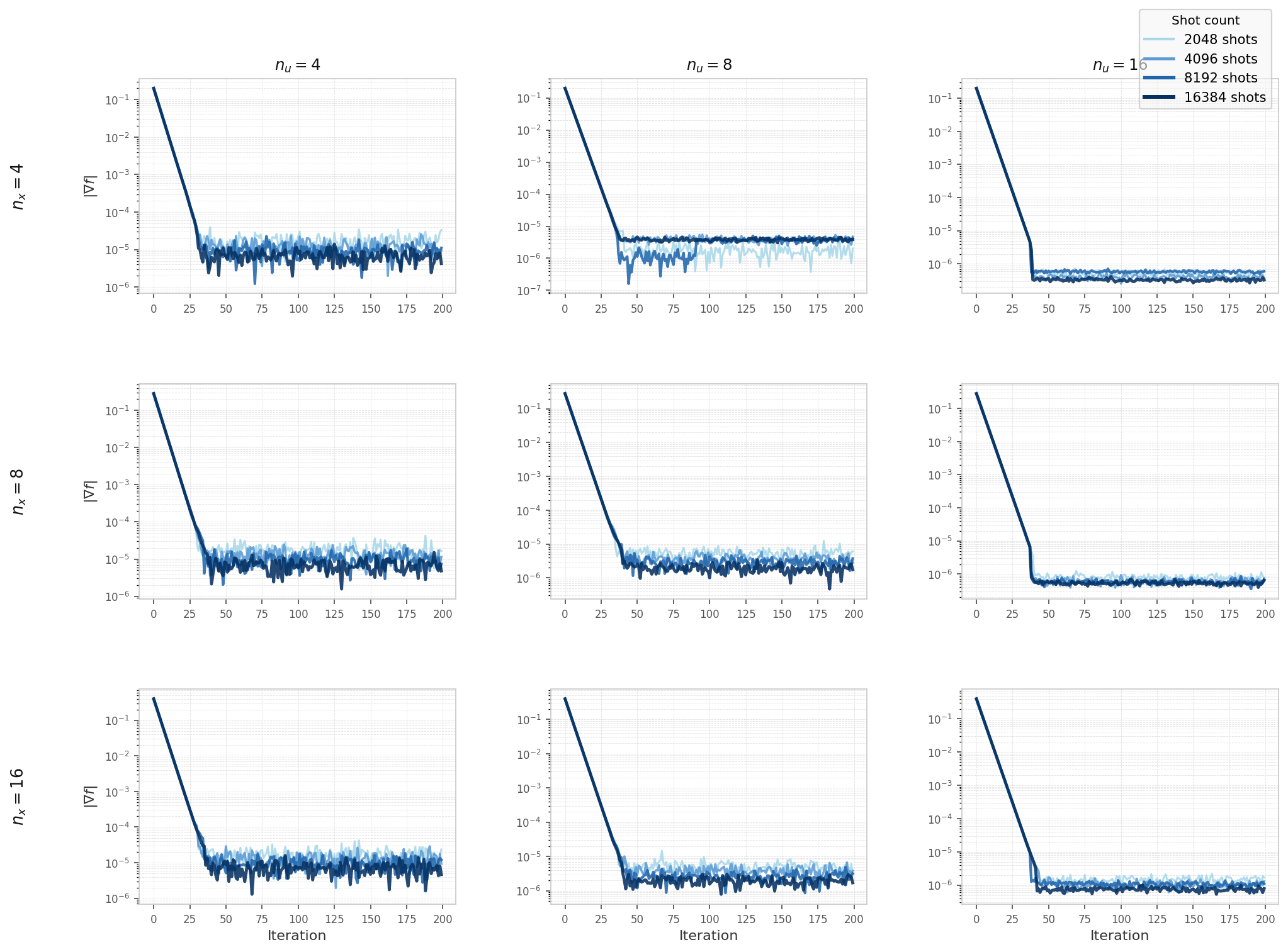
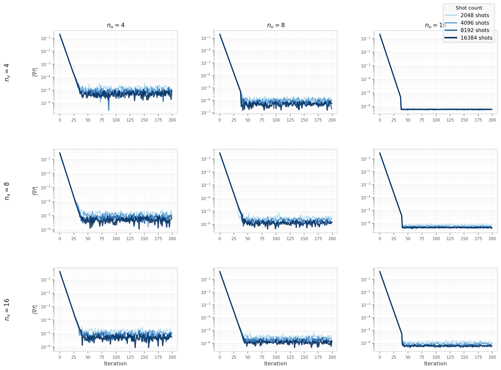
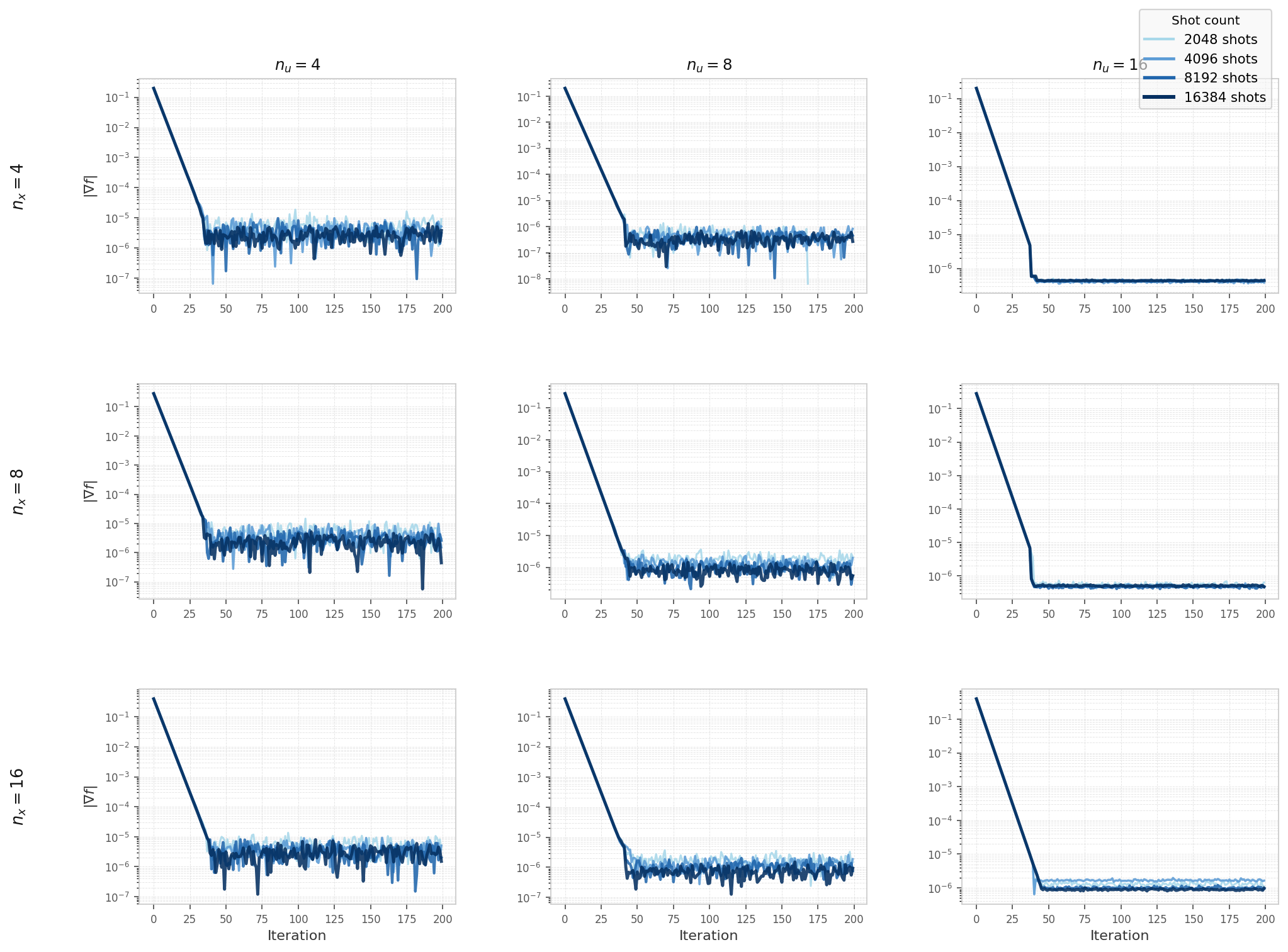
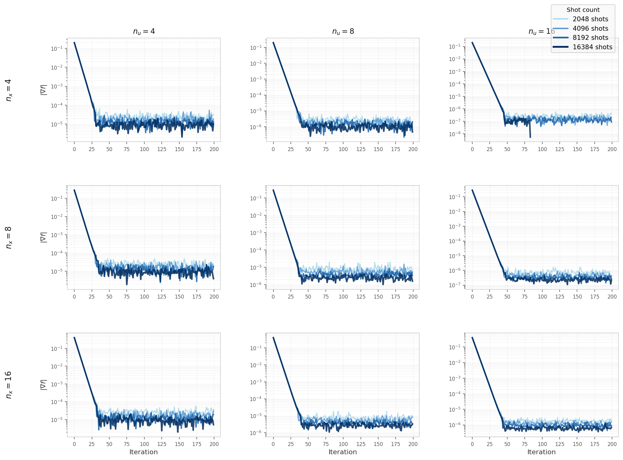
Hybrid solver convergence on the nonlinear heat equation (Qiskit Aer simulator), swept over
state-variable count nu ∈ {4, 8, 16} (columns), control-variable count
nx ∈ {4, 8, 16} (rows), and shot count ∈ {2048, 4096, 8192, 16384}.
All configurations converge to a shot-noise floor that is largely independent of problem size.
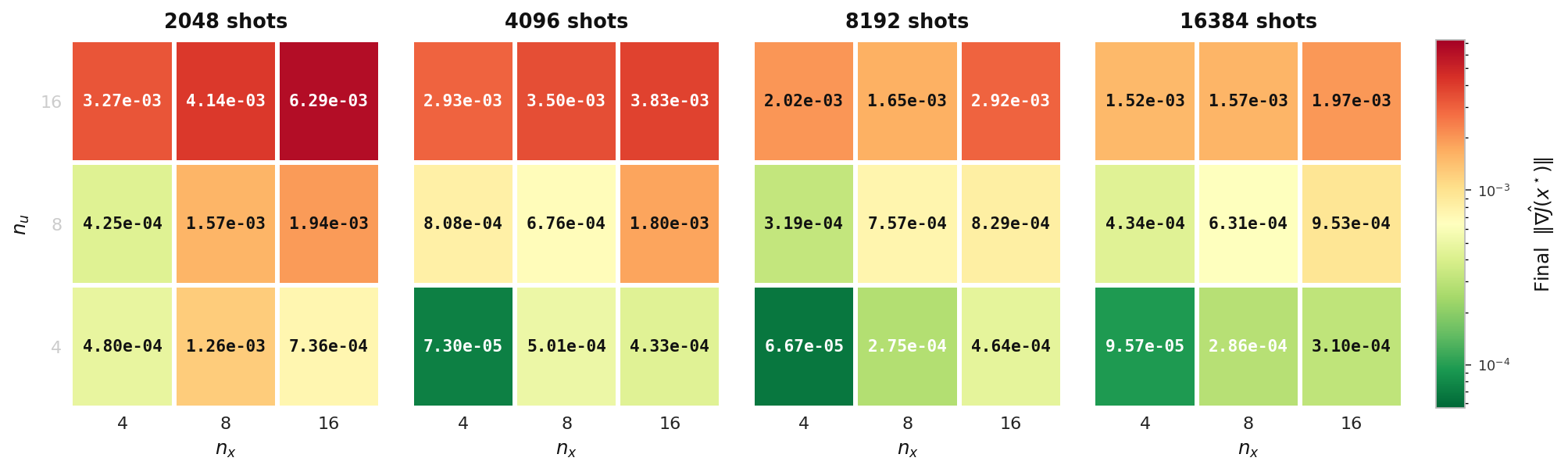
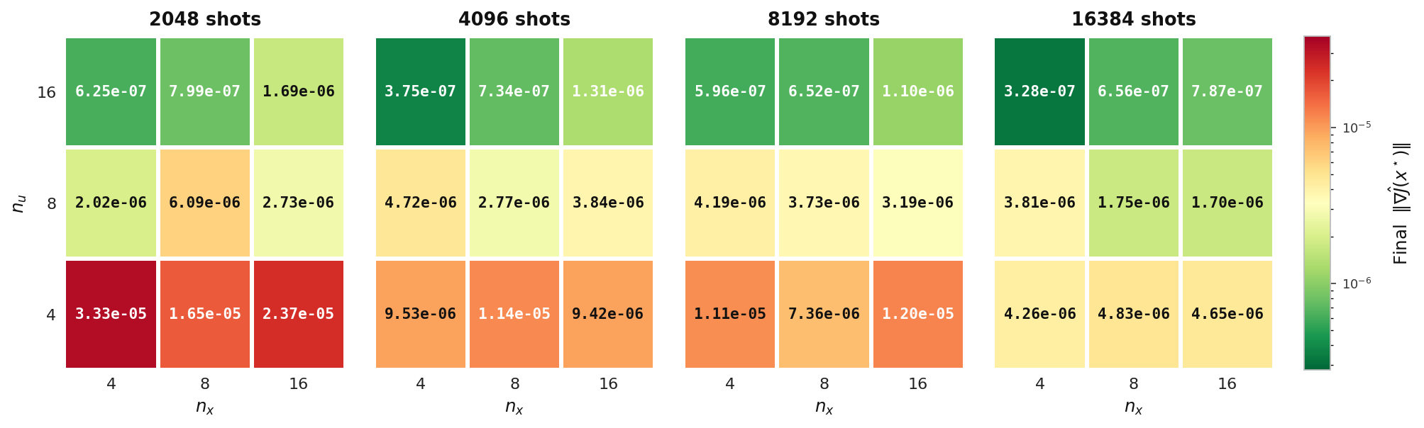
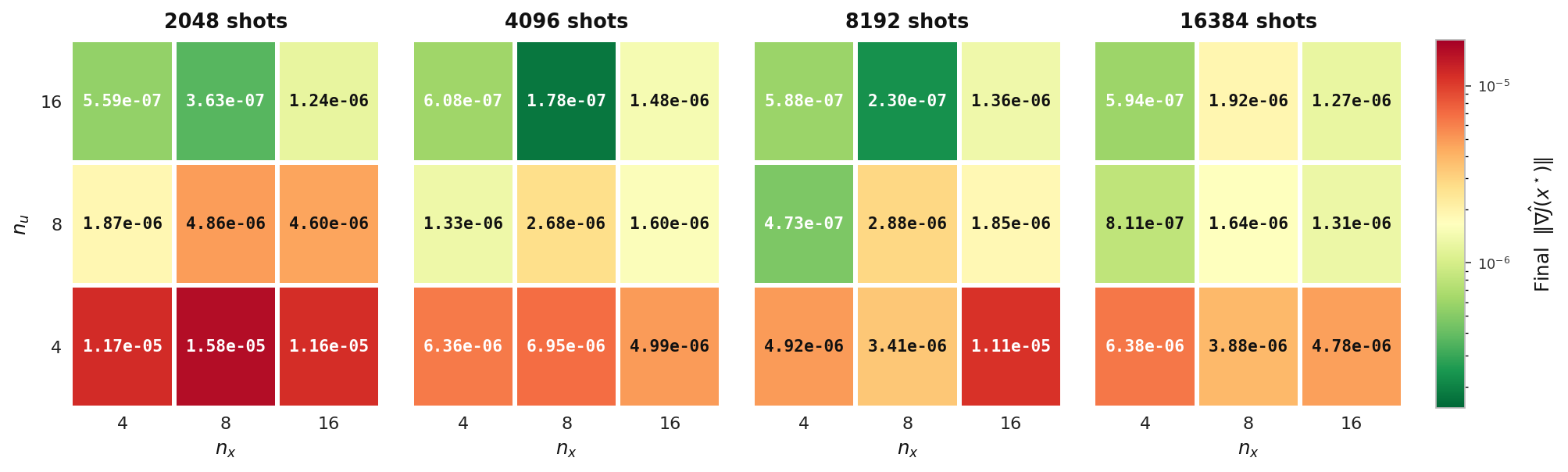
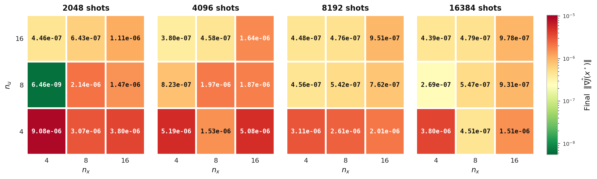
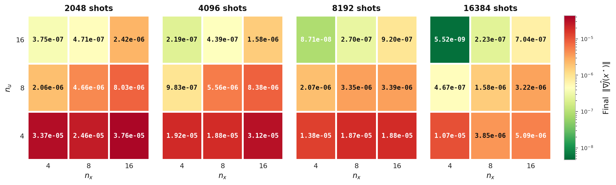
Final ‖∇Ĵ‖
Final gradient norm reached by the hybrid solver, tabulated over state count nu and control count nx, one panel per shot count. Lower (greener) values indicate a more fully converged optimum.
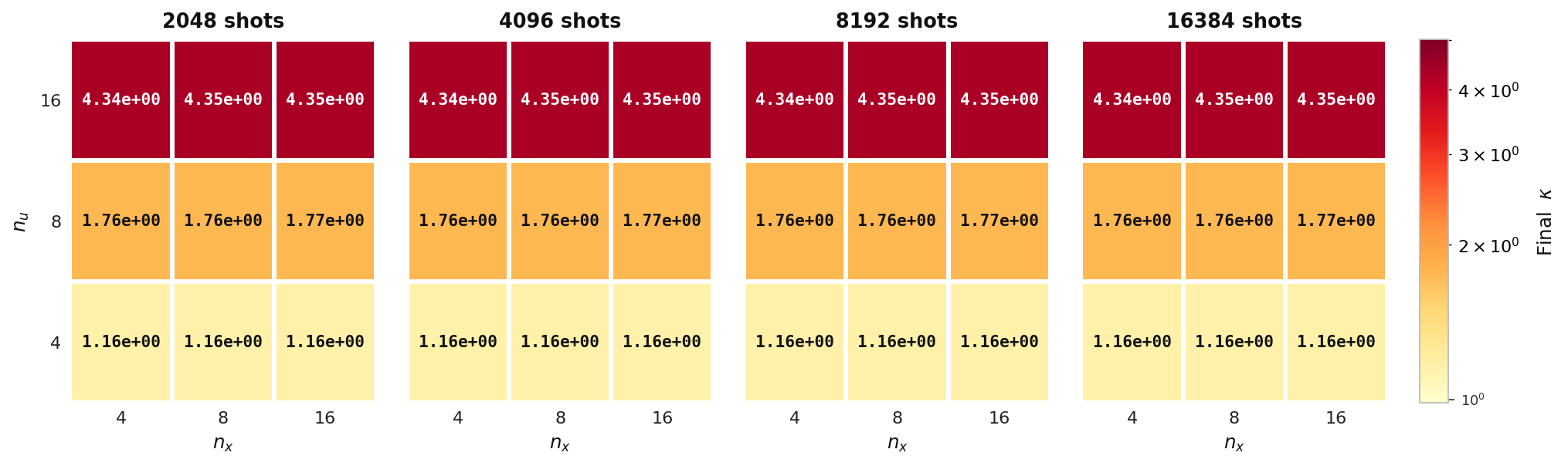
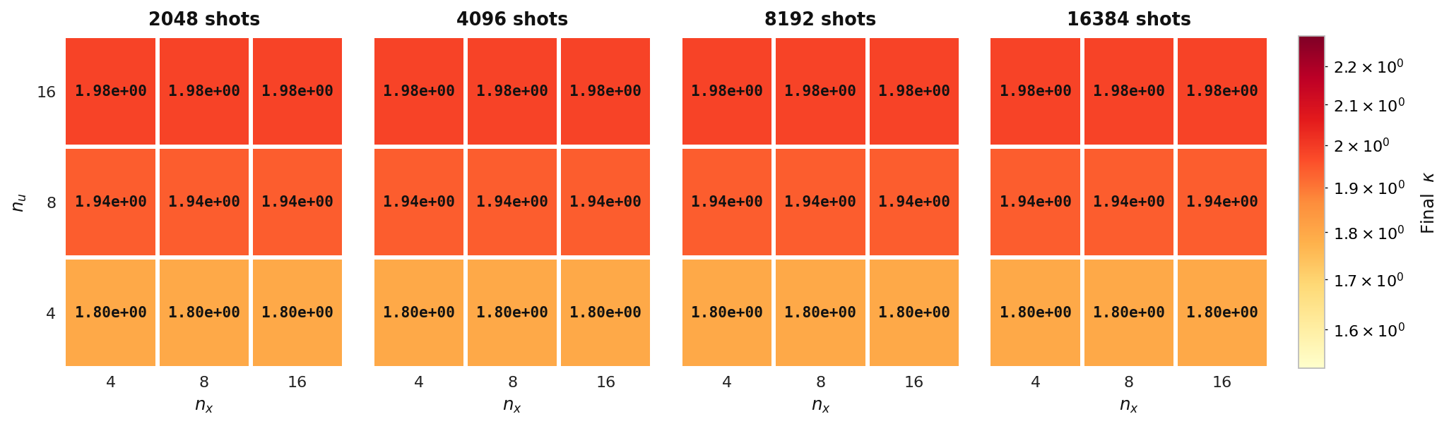
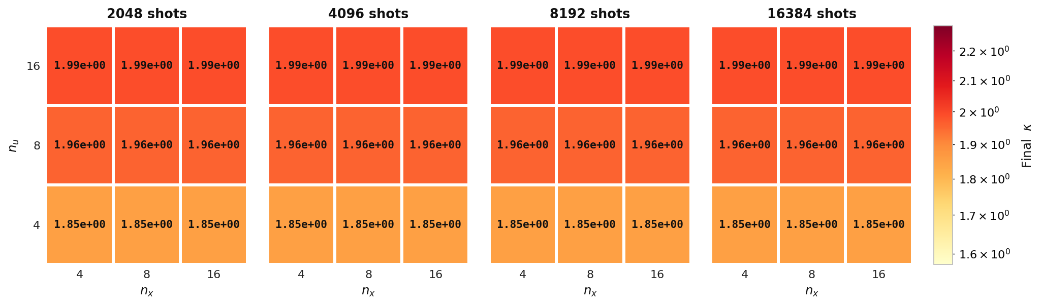
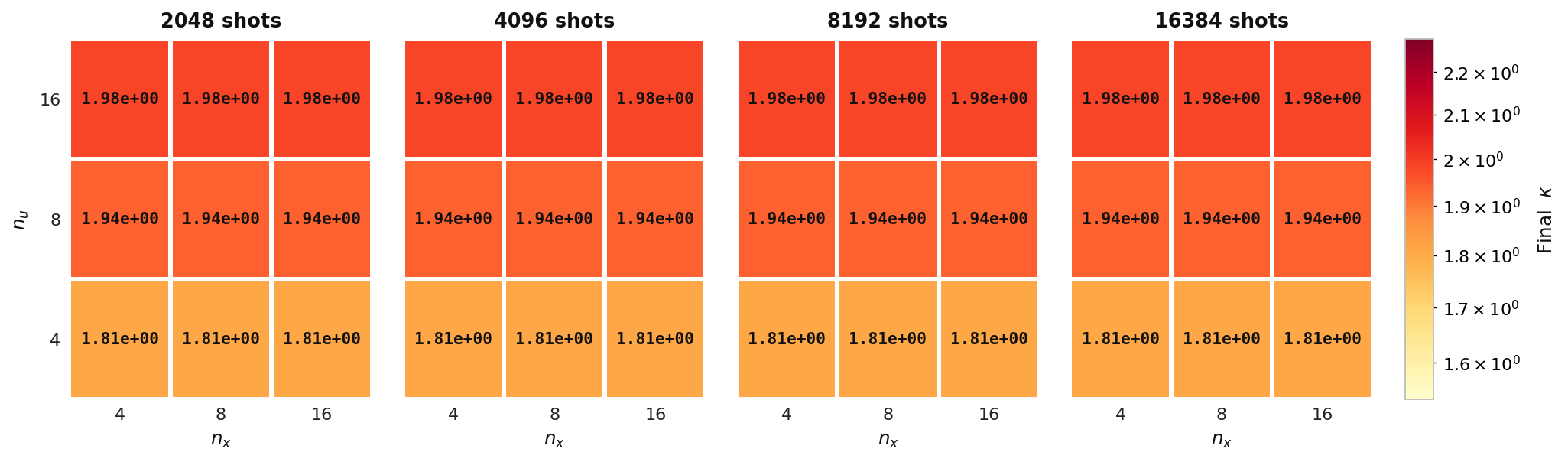
Final κ
Final adjoint condition number κ over the same (nu, nx) grid. κ stays essentially flat across shot counts, showing it is set by the PDE discretization rather than by the quantum measurement budget.
Final gradient norm and final adjoint condition number reached by the hybrid solver — heat model, Aer simulator.
Hybrid solver convergence on the elliptic model (Experiment 1, Qiskit Aer simulator), swept over
nu, nx, and shot count.
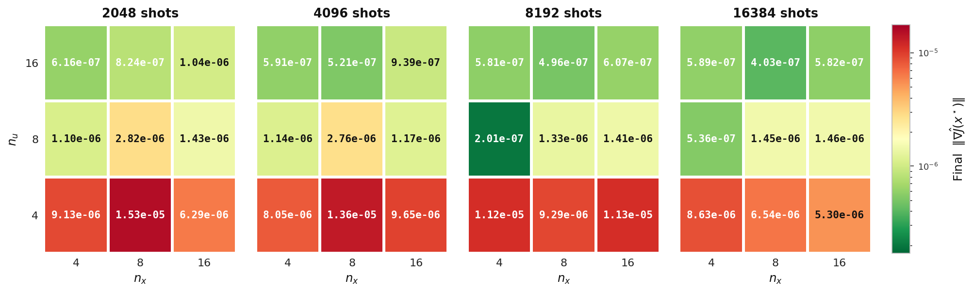
Final ‖∇Ĵ‖
Final gradient norm reached by the hybrid solver on the elliptic model (Experiment 1), tabulated over state count nu and control count nx, one panel per shot count. Lower (greener) values indicate a more fully converged optimum.

Final κ
Final adjoint condition number κ over the same (nu, nx) grid for Experiment 1. κ stays essentially flat across shot counts, showing it is set by the PDE discretization rather than by the quantum measurement budget.
Final gradient norm and final adjoint condition number — elliptic model, Experiment 1, Aer simulator.
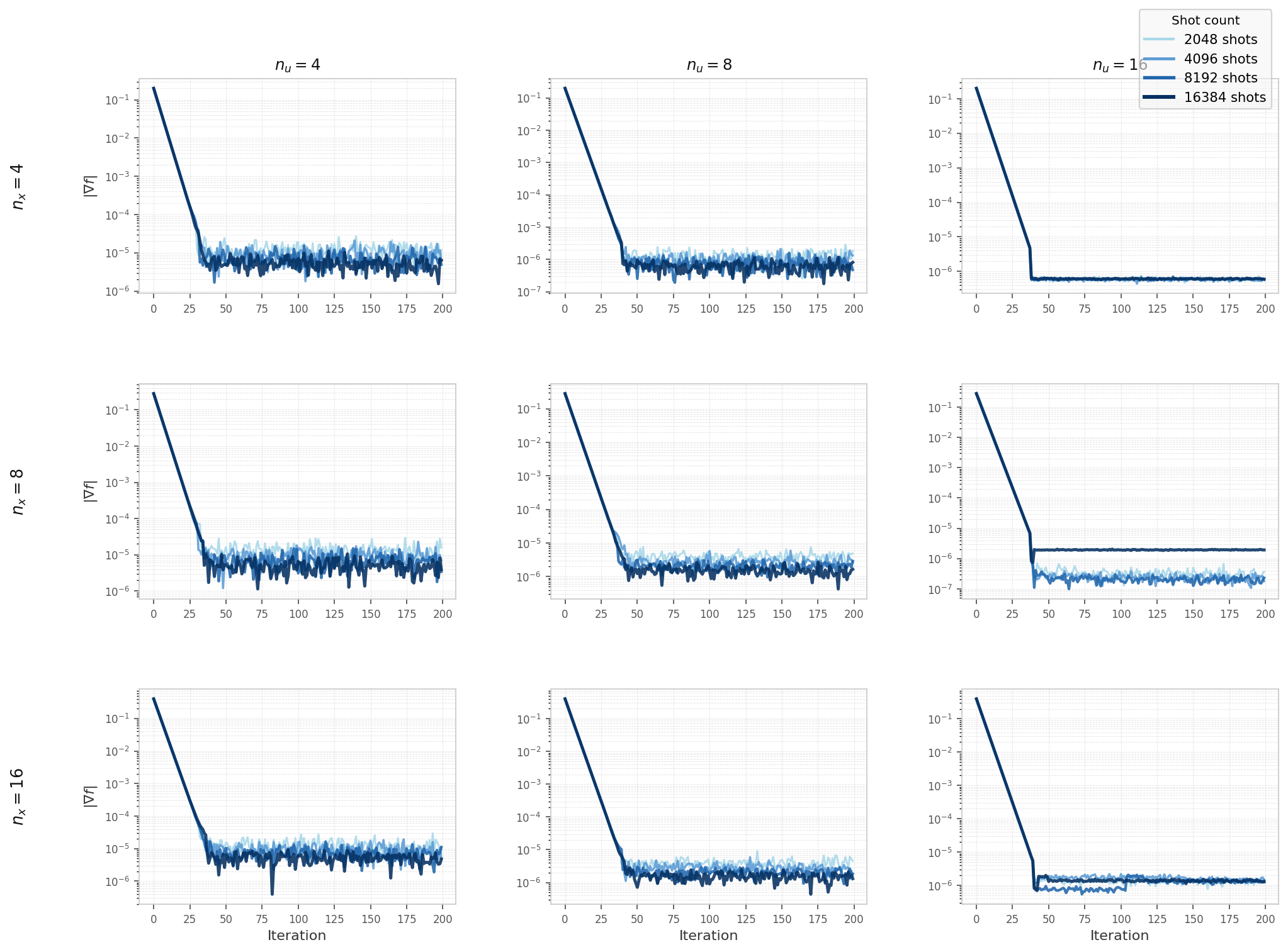
Hybrid solver convergence on the elliptic model (Experiment 2, Qiskit Aer simulator), swept over
nu, nx, and shot count.
Final ‖∇Ĵ‖
Final gradient norm reached by the hybrid solver on the elliptic model (Experiment 2), tabulated over state count nu and control count nx, one panel per shot count. Lower (greener) values indicate a more fully converged optimum.
Final κ
Final adjoint condition number κ over the same (nu, nx) grid for Experiment 2. κ stays essentially flat across shot counts, showing it is set by the PDE discretization rather than by the quantum measurement budget.
Final gradient norm and final adjoint condition number — elliptic model, Experiment 2, Aer simulator.
Hybrid solver convergence on the elliptic model (Experiment 3, Qiskit Aer simulator), swept over
nu, nx, and shot count.
Final ‖∇Ĵ‖
Final gradient norm reached by the hybrid solver on the elliptic model (Experiment 3), tabulated over state count nu and control count nx, one panel per shot count. Lower (greener) values indicate a more fully converged optimum.
Final κ
Final adjoint condition number κ over the same (nu, nx) grid for Experiment 3. κ stays essentially flat across shot counts, showing it is set by the PDE discretization rather than by the quantum measurement budget.
Final gradient norm and final adjoint condition number — elliptic model, Experiment 3, Aer simulator.
Hybrid solver convergence on the elliptic model (Experiment 4, Qiskit Aer simulator), swept over
nu, nx, and shot count.
Final ‖∇Ĵ‖
Final gradient norm reached by the hybrid solver on the elliptic model (Experiment 4), tabulated over state count nu and control count nx, one panel per shot count. Lower (greener) values indicate a more fully converged optimum.
Final κ
Final adjoint condition number κ over the same (nu, nx) grid for Experiment 4. κ stays essentially flat across shot counts, showing it is set by the PDE discretization rather than by the quantum measurement budget.
Final gradient norm and final adjoint condition number — elliptic model, Experiment 4, Aer simulator.
Hybrid solver convergence on the elliptic model (Experiment 5, Qiskit Aer simulator), swept over
nu, nx, and shot count.
Final ‖∇Ĵ‖
Final gradient norm reached by the hybrid solver on the elliptic model (Experiment 5), tabulated over state count nu and control count nx, one panel per shot count. Lower (greener) values indicate a more fully converged optimum.

Final κ
Final adjoint condition number κ over the same (nu, nx) grid for Experiment 5. κ stays essentially flat across shot counts, showing it is set by the PDE discretization rather than by the quantum measurement budget.
Final gradient norm and final adjoint condition number — elliptic model, Experiment 5, Aer simulator.
BibTeX
@article{YourPaperKey2024,
  title={Your Paper Title Here},
  author={First Author and Second Author and Third Author},
  journal={Conference/Journal Name},
  year={2024},
  url={https://your-domain.com/your-project-page}
}