Deutsch / Deutsch-Jozsa

n = 1 is Deutsch’s algorithm. n > 1 is Deutsch-Jozsa. Same code either way. The code lives in hsp/dj_hsp/.

The problem

You are given a function \(f: \{0,1\}^n \to \{0,1\}\) as a black box, with a promise: \(f\) is either

• constant – the same value for every input, or

• balanced – 0 for exactly half of the \(2^n\) inputs and 1 for the other half.

Classically, deciding which one it is can take up to \(2^{n-1}+1\) queries in the worst case. The quantum algorithm always decides it with one query to the oracle.

The oracle

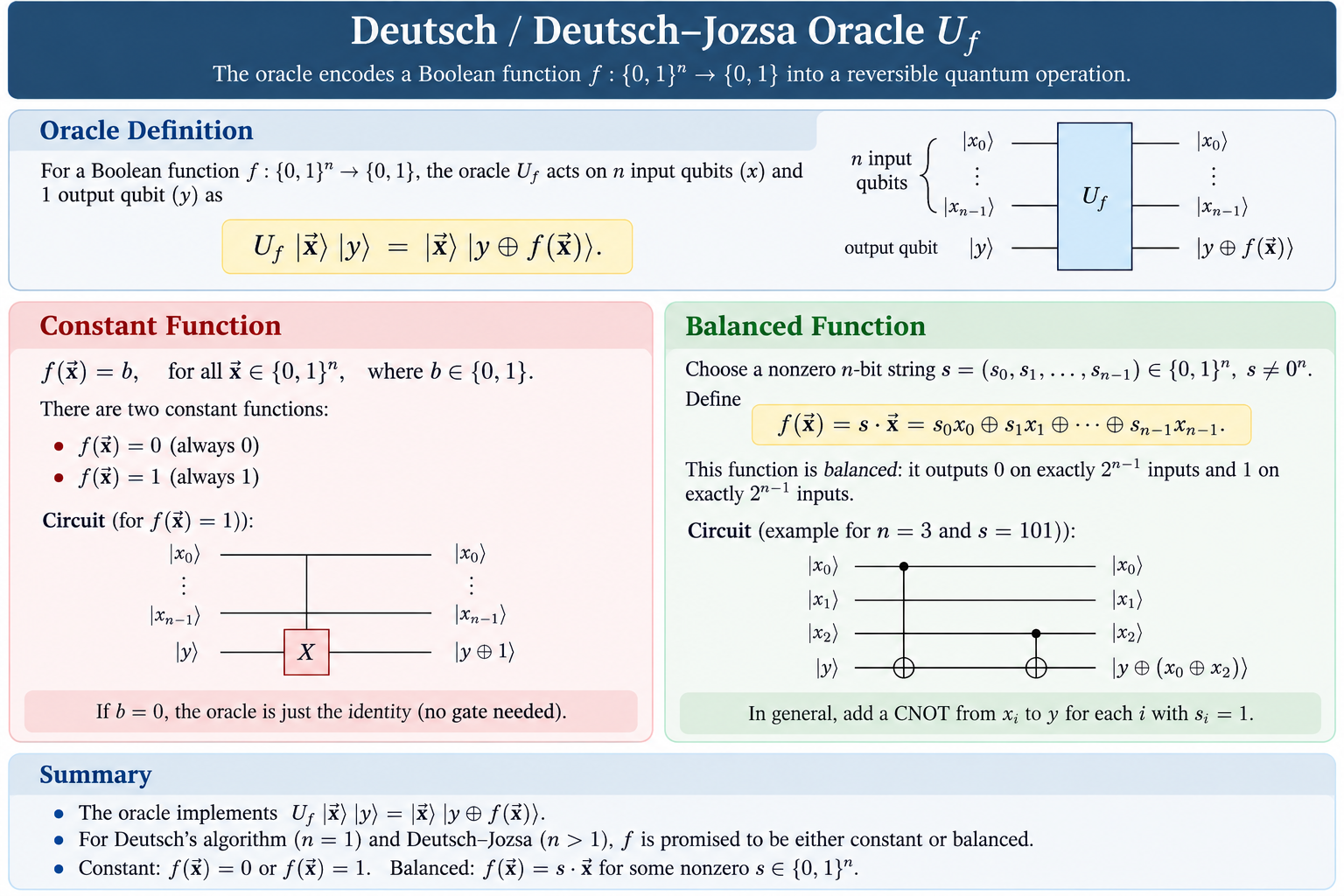
hsp/dj_hsp/oracle.py builds a reversible circuit U_f : |x>|y> -> |x>|y XOR f(x)> on n input qubits (x) plus 1 output qubit (y), via dj_oracle(n, kind, secret, constant_value, seed):

• kind="constant" – f(x) is the same value for every x. Built with an X on y (or nothing, for the all-zero case).

• kind="balanced" – f(x) is the XOR of the bits of x where a fixed nonzero string s has a 1. Built with one CNOT(x_i, y) per 1 bit in s. Flipping any input bit where s is 1 always flips the output, which pairs up all \(2^n\) inputs into 0/1 pairs – so this is balanced for any nonzero s, with nothing to check case by case.

These are the only two cases Deutsch-Jozsa’s promise allows, so kind accepts nothing else.

verify_promise() brute-force simulates the built circuit over all \(2^n\) inputs and confirms it really is constant or balanced. It runs automatically when you call oracle.py directly, for n up to 12.

The algorithm

hsp/dj_hsp/deutsch_jozsa.py wraps the oracle in the standard circuit:

x (n qubits): |0> --H--[ oracle ]--H--measure
y (1 qubit):  |0> --X----H---------[ oracle ]

y is prepared as \(|-\rangle\) (X then H), so the oracle leaves a phase \((-1)^{f(x)}\) on \(|x\rangle\) instead of flipping a qubit (phase kickback). After the second round of H gates on x:

• measuring all zeros means \(f\) is constant

• measuring anything else means \(f\) is balanced

run_deutsch_jozsa(n, kind, secret, constant_value, seed, shots, backend, memory) builds the oracle for that exact n, runs the circuit shots times on AerSimulator, and returns the verdict along with the measurement counts (and, with memory=True, every individual shot’s outcome). Because the same n builds both the oracle and the algorithm circuit, they can never end up sized differently.

run_shots_sweep(n, kind, secret, constant_value, seed, shots_list, backend) builds the oracle once and runs it at each shot count in shots_list, reporting what fraction of shots landed on the expected outcome (the oracle’s 0s for constant, the secret reversed for balanced) at each count – see Comparing accuracy across shot counts.

The classical solver

hsp/dj_hsp/classical.py solves the same problem with no circuit, no simulator, and no Qiskit involved in the decision at all: it evaluates f directly as plain Python, querying x = 0, 1, 2, ... in order and stopping the moment two different outputs turn up (f is balanced), or once \(2^{n-1}+1\) queries have all agreed (f is constant – see Why 2^(n-1)+1 queries are enough classically for why that many queries is enough).

run_classical_deutsch_jozsa(n, kind, secret, constant_value, seed) takes the same arguments as run_deutsch_jozsa (minus shots/backend, which have no classical meaning) and returns the same oracle metadata shape, plus every query made, how many queries that took, the worst-case bound, and the verdict – so a classical and a quantum run are easy to compare side by side.

Run it against the exact same config as run.py (the quantum-only fields – shots, backend, memory, shots_sweep – are ignored):

python hsp/dj_hsp/classical.py                     # uses config.yaml next to it
python hsp/dj_hsp/classical.py path/to/other.yaml

Deutsch-Jozsa algorithm, classical solver: n=4
oracle: kind=balanced  secret=0110
queries used: 3 (worst-case bound: 9 = 2^(n-1)+1, out of 2^n = 16 possible inputs)
result: f is BALANCED
(the quantum algorithm decides this with exactly 1 query, regardless of n)
saved: results/n4_balanced_classical_20260101T120000.json

When secret is left null, classical.py picks the same random secret from the same seed that oracle.py would, so pointing both scripts at one config.yaml tests the identical hidden oracle.

Why 2^(n-1)+1 queries are enough classically

A balanced f is 0 on exactly half of the \(2^n\) inputs and 1 on the other half (that is the promise). So no value can appear on more than \(2^{n-1}\) inputs if f is balanced. Querying \(2^{n-1}+1\) distinct inputs and seeing the same value on every one of them is therefore only possible if f is constant – by the pigeonhole principle. That is the deterministic classical algorithm’s worst case; the quantum algorithm needs exactly 1 query regardless of n.

Files

hsp/dj_hsp/
├── oracle.py          # dj_oracle() + verify_promise()
├── deutsch_jozsa.py   # build_circuit(), run_deutsch_jozsa(), run_shots_sweep()
├── classical.py       # classical_f() + run_classical_deutsch_jozsa(): the classical solver
├── run.py             # CLI: reads config.yaml, runs (or sweeps), saves results
└── config.yaml        # n, kind, secret, seed, shots, backend, memory,
                        # results_dir, shots_sweep

Configuration

One YAML file drives both the oracle and the algorithm (see Configuration with YAML):

n: 4               # input qubits (1 = Deutsch, >1 = Deutsch-Jozsa)
kind: balanced     # constant | balanced -- the only two cases the promise allows
constant_value: 0  # 0 or 1, used when kind=constant
secret: null       # n-bit binary string, used when kind=balanced
seed: 7            # picks a random secret when kind=balanced and secret is null
shots: 1024        # measurements for a single run (ignored if shots_sweep is set)
backend: aer_simulator
memory: false      # store every shot's individual outcome, not just aggregated counts
results_dir: results   # where run.py saves output; relative to the current directory,
                        # or an absolute path; set to null to not save anything
shots_sweep: null  # e.g. [64, 128, 256, 512, 1024] -- compare accuracy across shot
                    # counts instead of the single run above; see below

backend accepts aer_simulator (the default) or a specific AerSimulator method: statevector, density_matrix, stabilizer, matrix_product_state, extended_stabilizer, unitary, superop.

memory stores each shot’s own outcome (Qiskit’s per-shot readout), not only the aggregated counts. It lets you check that every shot really did agree, rather than trusting the counts dict alone.

results_dir is where run.py saves what it produced. Leave it as results (created next to wherever you run the command from), point it anywhere else, or set it to null to save nothing. Saving the exact config next to the result is the rule described on the configuration page.

Run it

With the qalgos environment active, from the repository root:

python hsp/dj_hsp/run.py                     # uses config.yaml next to run.py
python hsp/dj_hsp/run.py path/to/other.yaml

To inspect just the oracle circuit (with the brute-force promise check):

python hsp/dj_hsp/oracle.py

Reading the output

Deutsch-Jozsa algorithm: n=4  shots=1024  backend=aer_simulator
oracle: kind=balanced  secret=0110
measurement counts: {'0110': 1024}
result: f is BALANCED
(qiskit prints bitstrings with qubit 0 on the right, so this reads as the secret above reversed)
saved: results/n4_balanced_20260101T120000.json

The saved JSON has the config used, the oracle metadata, the counts, the verdict, and (if memory: true) every shot’s own outcome – everything needed to reproduce the run.

Comparing accuracy across shot counts

Set shots_sweep in the config to a list of shot counts instead of running once at shots:

shots_sweep: [64, 128, 256, 512, 1024, 2048]

run.py then builds the oracle once and runs it at each shot count, recording what fraction of shots measured the expected outcome:

Deutsch-Jozsa accuracy vs shots: n=4  kind=balanced  backend=aer_simulator
  shots=64       accuracy=1.0000  verdict=balanced
  shots=256      accuracy=1.0000  verdict=balanced
  shots=1024     accuracy=1.0000  verdict=balanced
saved: results/accuracy_vs_shots_n4_balanced_20260101T120000.xlsx

The .xlsx has one row per shot count (shots, accuracy, hits, verdict, distinct_outcomes, top_outcome); the config used is saved next to it as a matching .config.json.

In a noiseless simulation Deutsch-Jozsa is exact, so accuracy is 1.0 at every shot count – this is where the sweep is most useful once a noisy backend (density_matrix with a noise model, or real IBM hardware) is in the mix, to see how many shots it takes for the majority answer to become reliable.

Sweeping n and shots on a Slurm cluster

hsp/cluster/ generates and submits a whole grid of (n, shots) runs as separate Slurm jobs, one folder per combination, each with its own config.yaml, job.slurm and results. See Sweeping n and shots on a Slurm cluster.

Class demo configs

hsp/demo/ has four ready-made configs, one for each combination of algorithm and promise case, for showing both quantum and classical side by side in class:

hsp/demo/
├── deutsch_constant.yaml         # n=1, kind=constant
├── deutsch_balanced.yaml         # n=1, kind=balanced
├── deutsch_jozsa_constant.yaml   # n=4, kind=constant
└── deutsch_jozsa_balanced.yaml   # n=4, kind=balanced

python hsp/dj_hsp/run.py       hsp/demo/deutsch_jozsa_balanced.yaml   # quantum: 1 query
python hsp/dj_hsp/classical.py hsp/demo/deutsch_jozsa_balanced.yaml   # classical: up to 9 queries

All shots agree in this noiseless simulation – that is the point of the algorithm, one query settles it. The note about reversed bitstrings is a Qiskit display convention (qubit 0 is the rightmost character), not an error; if you compare the measured string to the secret printed above it, reverse one of them first.